How to replace estimations and guesses with a Monte Carlo simulation
There are many ways of estimating how long a software project will take. All of them are a waste of time.
Some prefer to spend days analysing and planning their changes so that they can estimate more accurately — others choose to multiply by N whatever estimations they make. I wouldn't recommend any of these approaches.
The problem with the first approach is that it considers software development to be a deterministic process when, in fact, it's stochastic. In other words, you can't accurately determine how long it will take to write a particular piece of code unless you have already written it.
The problem with multiplying estimations by N is that you're simply exchanging cycle time for predictability. Instead of actually trying to be accurate, you're merely adding a buffer to your estimations. That buffer wouldn't be a problem if it weren't for the fact that engineers determine it by licking the tip of their finger and putting it up in the air.
Unfortunately, the only way to win at the estimation game is not to play it.
To learn more these types of problems, see Gordian Knot and The most efficient way to solve problems.
“Estimation is a waste of time. Don’t do it.”
— VACANTI, Daniel.
Instead of making "informed" guesses or multiplying estimations by N, we can embrace the randomness and variability involved in writing software and use more suitable statical methods, in this case, stochastic modeling techniques, to devise better forecasts. One of these techniques is the Monte Carlo method, which I’ll use to make projections in the rest of this post.
This post will teach you how to replace estimations and guesses with a Monte Carlo simulation.
First, I’ll explain what is the Monte Carlo method and show how it works. Then, I will demonstrate how you could use it to forecast when a project is likely to be finished.
In the third section of this blog post, I’ll show you how to attach a probability value to your projections, turning them into actual forecasts¹. In this section, you’ll understand how to generate more or less optimistic forecasts depending on your risk appetite.
After those first three sections, I’ll explain a few caveats and factors to which you should pay attention when running your Monte Carlo simulations to generate projections.
At last, explain where we’ll go in the next blog posts and recommend further reading material.
What is the Monte Carlo method?
The Monte Carlo method consists of repeatedly simulating random individual events to understand the likelihood of possible outcomes.
Imagine, for example, that you’d like to calculate the likelihood of rolling two dice and obtaining a sum of seven.
One of the ways of doing it is to enumerate all the 36 possible result combinations and count how many of those results yield a sum of seven. Considering 6 of those 36 results produce a sum of 7, the probability of rolling a seven is 16.67%.
Alternatively, you could roll two dices for the next couple of months, take notes of all the results, and check how often you rolled a seven. The more rolls you’ve made, the more precise your final probability estimation will be.
Now, rolling dice for days isn’t very exciting (and takes too long). Instead, we could get the computer to roll the dice for us. Thanks to the machines, we can roll two dice a million times quite quickly.
Now, let’s write a simple Rust program to roll two dice a million times and tell us how often it rolls a seven.
extern crate rand;

use rand::distributions::{Distribution, Uniform};
use rand::thread_rng;

const TOTAL_ROLLS: i32 = 1_000_000;

fn main() {
    let mut rng = thread_rng();
    let die = Uniform::from(1..7);

    let mut sevens = 0;
    for _ in 0..TOTAL_ROLLS {
        let first_die = die.sample(&mut rng);
        let second_die = die.sample(&mut rng);
        if first_die + second_die == 7 {
            sevens += 1
        }
    }

    let p: f64 = f64::from(sevens) / f64::from(TOTAL_ROLLS) * f64::from(100);

    println!("Total Rolls: {}", TOTAL_ROLLS);
    println!("Total Sevens: {}", sevens);
    println!("Probability of rolling a seven: {:.2}%", p);
}
When running this program, it'll simulate a million dice rolls, divide the number of sevens rolled by the total number of simulations, and output the empirical probability of rolling a seven. This probability will be close to 16.67%, which is the actual probability of rolling a seven.
Total Rolls: 1000000
Total Sevens: 166446
Probability of rolling a seven: 16.64%
Congratulations, you just did your first Monte Carlo simulation.
Simulating when a project will be complete
Now that you’ve done a Monte Carlo simulation, I’ll teach you how to apply the same principles to a software project so that you can estimate when you’ll complete it.
Let’s imagine you’ve read a Tim Ferris blog post saying that the optimal number of blog posts a year is 60 or more. Because it’s Tim Ferriss, you’re convinced he’s right, and you’d like to follow his advice.
However, before you commit to this time-consuming endeavour, you want to know how likely you are to be able to write 60 or more posts in 365 days and, if not, what changes you could make to hit that mark. How can we do that?
A naive approach: uniformly distributed cycle-times
First, we’ll take a naive approach: we’ll assume you know how long it took to write each of the blog posts you published in the past three months. For the sake of this example, let’s say that the shortest post took two days to complete, and the longest took ten.
Then, we’ll pretend that you’re equally likely to complete posts in any number of days between two and ten. To put it another way, we’ll consider your posts’ cycle-time distribution to be uniform (just like a die).
Considering these assumptions would hold, you could write a program to repeatedly simulate how long it would take to write 60 blog posts.
In this simulation, for each blog post, your program would randomly pick a number between two and ten as if that were the number of days you took to write it.
After simulating how long each post took to write, your program would sum each post’s turnaround and check whether all 60 posts took less than 365 days.
Finally, once it has run all the simulations, your program would calculate the probability of success by dividing the number of times you “succeeded” by the total number of simulations.
extern crate rand;

use rand::distributions::{Distribution, Uniform};
use rand::thread_rng;

const TOTAL_RUNS: i32 = 1_000_000;
const TOTAL_BLOG_POSTS: i32 = 60;

fn main() {
    let mut rng = thread_rng();
    let time_to_completion = Uniform::from(2..11);

    let mut successes = 0;

    for _ in 0..TOTAL_RUNS {
        let mut current_duration = 0;

        for _ in 0..TOTAL_BLOG_POSTS {
            current_duration += time_to_completion.sample(&mut rng);
        }

        if current_duration <= 365 {
            successes += 1
        }
    }

    let p = f64::from(successes) / f64::from(TOTAL_RUNS) * f64::from(100);

    println!("Total Simulations: {}", TOTAL_RUNS);
    println!("Successes: {}", successes);
    println!("Probability of succeeding: {:.2}%", p);
}
After running this program, you should see an output similar to this:
Total Simulations: 1000000
Successes: 608671
Probability of succeeding: 60.87%
That’s a great first attempt, but let’s say it doesn’t feel quite right to you. What could you do to make your simulation more accurate?
An okay approach: weighted probabilities
Now, assume that, even though the shortest story took two days and the longest took ten, you remembered that the time for most posts skews towards the ten-day mark.
In other words, you don’t think that the posts cycle times are uniformly distributed: most posts take a long time, and only a few take two or three days.
In an attempt to make the model more accurate and get a more realistic forecast, you then gather the start and end date of each post and calculate each post’s cycle time.
| N | Title | Start Date | End Date | Time Taken |
|---|---|---|---|---|
| 1 | Why Your Software Never Works Out the Way You Plan | 12/01/2022 | 19/01/2022 | 8 |
| 2 | Ways Your Mother Lied to You About Software | 21/01/2022 | 29/01/2022 | 9 |
| 3 | A Software Success Story You’ll Never Believe | 02/02/2022 | 03/02/2022 | 2 |
| 4 | Darth Vader’s Guide to Software | 18/02/2022 | 23/02/2022 | 6 |
| 5 | How to Win Big in the Software Industry | 24/02/2022 | 29/02/2022 | 6 |
| 6 | Why Do People Think Software is a Good Idea? | 01/03/2022 | 08/03/2022 | 8 |
| 7 | Shocking Ways Software Will Make You a Better Dancer | 09/03/2022 | 12/03/2022 | 3 |
| 8 | What The Beatles Could Learn from Software | 14/03/2022 | 23/03/2022 | 10 |
| 9 | What Your Parents Never Told You About Software | 23/03/2022 | 28/03/2022 | 6 |
| 10 | How To Create The Worst Blog Post Titles | 28/03/2022 | 31/03/2022 | 4 |
With this data, you can now calculate the probability of each duration occurring and build a table like the one below.
| Duration | Frequency | Probability |
|---|---|---|
| 10 | 1 | 10% |
| 9 | 1 | 10% |
| 8 | 2 | 20% |
| 6 | 3 | 30% |
| 4 | 1 | 10% |
| 3 | 1 | 10% |
| 2 | 1 | 10% |
Knowing how likely each duration is to occur will make your simulation much more accurate.
In the naive approach you’ve just seen, an issue was equally likely to last two, six, or eight days, which doesn’t reflect reality.
By looking at the table above, you can easily see that tasks are three times more likely to take six days than two days. In fact, only 30% of stories take four days or fewer.
Now, let’s update our simulation so that it will obey the probability of each duration occurring.
extern crate rand;

use rand::distributions::{Distribution, Uniform};
use rand::thread_rng;

const TOTAL_RUNS: i32 = 1_000_000;
const TOTAL_BLOG_POSTS: i32 = 60;

const DURATIONS: [i32; 10] = [2, 3, 4, 6, 6, 6, 8, 8, 9, 10];

fn main() {
    let mut rng = thread_rng();
    let time_to_completion = Uniform::from(0..DURATIONS.len());

    let mut successes = 0;

    for _ in 0..TOTAL_RUNS {
        let mut current_duration = 0;

        for _ in 0..TOTAL_BLOG_POSTS {
            let random_index = time_to_completion.sample(&mut rng);
            current_duration += DURATIONS[random_index];
        }

        if current_duration <= 365 {
            successes += 1
        }
    }

    let p = f64::from(successes) / f64::from(TOTAL_RUNS) * f64::from(100);

    println!("Total Simulations: {}", TOTAL_RUNS);
    println!("Successes: {}", successes);
    println!("Probability of succeeding: {:.2}%", p);
}
After running this simulation, which is much more accurate, it’ll tell you that you’re actually 36.69% likely to succeed. That’s almost half of the previous estimation!
Total Simulations: 1000000
Successes: 366944
Probability of succeeding: 36.69%
This estimation is probably good enough for a single person, but it won’t work for a team. At least not without adjustments².
The problem with this simulation is that it assumes that blog posts will be written in series, not in parallel.
If you had two or more people working in parallel, you’d have to record their individual cycle times, simulate how many blog posts each one could write in 365 days, and sum each person's output.
Not too difficult, but there is an easier way.
Sampling throughput
An easier way of simulating a team’s performance without using individuals' cycle times is to sample the team’s throughput for each day in the simulation.
To perform such a simulation, you need to record the daily number of completed items for a determined length of time. With that data, you’d then have the probability of having a throughput of 0, 1, 2, 3, or more items on any given day, which you’d use when sampling.
If you were to write a program that did exactly that, you’d have a piece of code like the one below.
extern crate rand;

use rand::distributions::{Distribution, Uniform};
use rand::thread_rng;

const TOTAL_RUNS: i32 = 1_000_000;
const TOTAL_STORIES: i32 = 500;

const TEN_DAY_THROUGHPUTS: [i32; 10] = [1, 2, 0, 1, 1, 2, 3, 1, 2, 1];

fn main() {
    let mut rng = thread_rng();
    let throughput = Uniform::from(0..TEN_DAY_THROUGHPUTS.len());

    let mut successes = 0;

    for _ in 0..TOTAL_RUNS {
        let mut stories_completed = 0;

        for _ in 0..366 {
            let random_index = throughput.sample(&mut rng);
            stories_completed += TEN_DAY_THROUGHPUTS[random_index];
        }

        if stories_completed > TOTAL_STORIES {
            successes += 1
        }
    }

    let p = f64::from(successes) / f64::from(TOTAL_RUNS) * f64::from(100);

    println!("Total Simulations: {}", TOTAL_RUNS);
    println!("Successes: {}", successes);
    println!("Probability of succeeding: {:.2}%", p);
}
You could use this approach to determine whether a software development team could finish a particular number of items within a specific period.
Caveats to pay attention to when building Monte Carlo simulations
Before claiming that the simulation above is reliable, I must expose a few things you’ll need to pay attention to when using a Monte Carlo Simulation to make forecasts:
- The quality of the inputs upon which your simulations depend.
- The consistency and predictability of your team.
- The need to re-forecast.
- The size of your work packages.
Quality of the inputs
Assume you had a team of ten engineers last year, but half of them quit the company three months ago. If you were to simulate how long this team would take to complete a project, you should not use throughput data from more than three months ago.
If you use a 10-engineer team’s throughput data to forecast the performance of a 5-engineer team, you will get over-optimistic results.
Similarly, if your team doubles in size, your simulation should not use historical data from when you had half the number of people. In this case, you also can't just assume projects will take half the time because it's extremely unlikely that productivity will scale linearly as you hire more developers.
Additionally, other factors like holidays or a massive rewrite can impact your input data.
Your team’s throughput between Christmas and New Year’s Eve, for example, will probably not be the same as the team’s throughput in February. Similarly, a massive rewrite that drastically increases how easy it is to change and extend your software will have an equally dramatic impact on your cycle times.
As Daniel Vacanti explains in When Will It Be Done?, _ “the fundamental assumption that the Monte Carlo Simulation is making is that the future you’re trying to predict looks roughly like the past you have data for “_.
Consistency and predictability
Our simulation will work just fine for the circumstances above because I came up with more predictable throughput values.
The range of throughputs used in that code is small, and, most of the days, the team is highly consistent: it gets one or two items done. In other words, the standard deviation for this cycle-time distribution is small.
In another blog post, I’ll explain what would have happened if I had used more erratic throughput values in the previous section. For now, keep in mind that as long as you have a team with consistent throughput, this simulation will be reliable.
Quantifying "predictability" and "consistency" is also a topic for another blog post.
Re-forecast!
As your project advances, you will encounter delays, and, sometimes, you’ll get to be ahead of schedule. Therefore, re-forecasting as you progress will make your forecast more accurate because there will be fewer items and more data and, consequently, less room for error.
The more information and fewer items to simulate you have, the more your forecast will converge to reality.
Guessing who’ll win the Premier League before it starts is much more difficult than guessing the winner halfway in, for example.
When the league starts, you have many games to simulate, so you have more room for error.
At that time, you also don't have data that reflects the current lineup performance. Imagine forecasting Barcelona's performance in 2021 using last year's lineup, for example. It certainly won't be the same without Messi.
Re-forecasting is also important to remain agile.
Suppose you forecast only once at the beginning of your project and create a Gantt chart based on those estimations. In that case, you’ll simply be running a waterfall process with statistically accurate dates.
In an agile context, as you re-run these simulations, you will be able to adapt your plan and processes based on results that will be increasingly more accurate as reality converges with the estimated results.
To summarise: the fewer days and items you have to simulate, the smaller the error margin.
Sizing work
At the beginning of this blog post, I claimed that a statistical approach could do away with all estimations.
Even though that is technically true given you won't have to assign story points to anything anymore (nor make informed guesses), throughput-based simulations assume that work items are roughly the same size. Therefore, one could claim that making work packages approximately the same size is another form of estimation.
Despite that claim, these statistical approaches still yield much better results because outliers won't significantly impact your simulation.
Additionally, you won't need to waste time discussing whether something is worth two or three story points. Instead, you can always try to make stories as small as you can so that you have more revealing data.
Using Monte Carlo Simulations in practice: confidence intervals
In the real world, we’re seldom looking for the probability of a project succeeding within a particular time frame. Instead, we’re looking to understand the possible scenarios in which we could end up and how likely those scenarios are to happen. In other words, we want to know how our simulation’s outcomes are distributed and attach "confidence" values to our forecasts.
When it comes to visualising an outcome distribution, a histogram is an excellent visual tool. Furthermore, the histogram’s underlying data will allow us to attach confidence values to our forecasts.
To demonstrate how you could use histograms in practice, let’s imagine your company needs to deliver a project of about 50 stories³. For the project to succeed, your company wants you to forecast an end date so that the marketing and sales teams can prepare for the launch. Considering how critical marketing is for this important product to succeed, executives want you to be pretty sure of whatever forecast you make.
Now, let’s try to solve this problem and come up with a precise forecast.
Given you want to play on the safe side, let’s define a “precise” forecast as a forecast in which you’re at least 95% confident.
First, we’ll adapt our code to generate histograms that show the dates on which the project is likely to finish.
Go ahead and update the code to store the number of times each date appeared in your simulations.
extern crate rand;

use rand::distributions::{Distribution, Uniform};
use rand::thread_rng;
use std::collections::HashMap;

const TOTAL_RUNS: i32 = 1_000_000;
const STORIES_TARGET: i32 = 50;
const TEN_DAY_THROUGHPUTS: [i32; 10] = [1, 2, 0, 1, 1, 2, 3, 1, 2, 1];

fn main() {
    let mut rng = thread_rng();
    let throughput = Uniform::from(0..TEN_DAY_THROUGHPUTS.len());

    let mut outcomes: HashMap<i64, i32> = HashMap::new();

    let one_day = Duration::days(1);

    let start_date: DateTime<Local> = Local::now();

    for _ in 0..TOTAL_RUNS {
        let mut current_date = start_date;
        let mut stories_completed = 0;

        while stories_completed < STORIES_TARGET {
            let random_index = throughput.sample(&mut rng);
            stories_completed += TEN_DAY_THROUGHPUTS[random_index];
            current_date = current_date + one_day;
        }

        let count = outcomes.entry(current_date.timestamp()).or_insert(0);
        *count += 1;
    }

    println!("Total Simulations: {}", TOTAL_RUNS);
}
As you can see in the code above, we are not targeting a particular outcome anymore. Instead, we are keeping track of how often the project ended on a specific date.
Remember: we want to understand how likely each delivery date is to come true so that we can make a forecast in which we’re 95% confident.
After this change, we’ll write a function that uses the plotters crate to generate a histogram and save it to disk. This histogram will display possible delivery dates on its X-axis and the number of times each delivery date came out in the simulations.
The plotting function is reasonably long, and not really interesting for what we're doing here, so I'll omit it from this post. If you still wanna see it, have a look at this post's related GitHub repository.
After running the simulation, your program should yield a histogram similar to the one below.
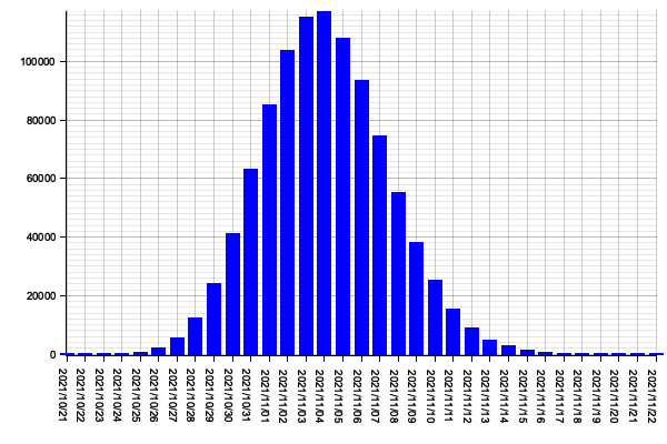
Looking at this histogram, you can clearly see that if we start working on the project’s 50 stories today (29th of September of 2021), the most likely date on which we’d finish it would be the 4th of November of 2021.
If this weren't an important project for which the company needs a precise forecast, you could tell executives that the 4th of November of 2021 is your best guess for the project’s end date.
Unfortunately, you were asked to offer a precise forecast, so you can’t simply provide the most likely end date. Instead, you’ll need to deliver a forecast in which you’re at least 95% confident.
To generate a forecast in which you’re at least 95% confident, you need to define what “95% confidence” means in terms of our Monte Carlo simulation. In this case, you could say that you’d be 95% confident in a particular end date if, in 95% of all the simulations, you finished the project on or before that date.
If, for example, you simulated a particular project a hundred times and in 95 of those simulations you finished the project on or before the 1st of April, then you’d be 95% confident that you could complete the project on or before that date.
For those more familiar with statistics, these are merely percentiles. A percentile is a value at or below which a particular percentage of the distribution’s values falls (considering an inclusive definition).
Let’s go ahead and create a function to calculate the 95th percentile for our simulation. This percentile will indicate the date at or before 95% of the simulations have finished. Therefore, we can say we’re “95% confident” that this will be the project’s end date.
fn calculate_percentile(data: &HashMap<i64, i32>, percentile: i32) {
    let total_sims: i32 = data.values().sum();

    let p_qtd: i32 = total_sims - (total_sims as f64 / (100_f64 / percentile as f64)).ceil() as i32;

    let mut hash_vec: Vec<(&i64, &i32)> = data.iter().collect();
    hash_vec.sort_by(|a, b| b.0.cmp(a.0));

    let mut sum = 0;
    let mut percentile_timestamp: i64 = 0;

    for (timestamp, freq) in hash_vec {
        sum += freq;

        if sum >= p_qtd {
            percentile_timestamp = *timestamp;
            break;
        }
    }

    println!(
        "Percentile {}: {} ({}/{})",
        percentile,
        Local
            .timestamp(percentile_timestamp, 0)
            .format("%Y/%m/%d")
            .to_string(),
        sum,
        total_sims
    );
}
Once you’ve created this function, update your program so that it calls calculate_percentile passing the histogram’s data and 95 as the percentile in which you’re interested. Doing this change and re-running will yield results similar to the following:
Total Simulations: 1000000
Percentile 95: 2021/11/13 (60032/1000000)
After seeing the program’s output, you know that 95% of your simulations finished on or before the 13th of November. Consequently, you can go back to the company’s executives and tell them that you’re 95% confident that the project will finish on or before that date.
Now, imagine that your company’s executives told you that they’d like to understand the likelihood of your project finishing on other dates. With that data, they could decide whether to hire more marketing professionals to prevent the product from being held up in case you finish writing the code earlier.
To provide your executives with that data, you can simply add a few more calls to calculate_percentile to calculate the 25th, 50th, 75th, 85th percentiles. These would be the dates on which or before 25%, 50%, 75%, and 85% of the simulations fall, respectively. Therefore, these are the final dates in which you could say you’re 25%, 50%, 75% and 85% confident.
Total Simulations: 1000000
Percentile 25: 2021/11/05 (765267/1000000)
Percentile 50: 2021/11/07 (546177/1000000)
Percentile 75: 2021/11/09 (320170/1000000)
Percentile 85: 2021/11/11 (152931/1000000)
Percentile 95: 2021/11/13 (59527/1000000)
As an exercise, I’d also recommend the reader to plot these percentiles in their histograms. This author would be interested in seeing your solution as he’s given up on doing that after an arduous battle with Plotters and the Rust compiler.
On forecasting based on your risk appetite
Once you know how likely it is for an event to happen, you can gauge or risk appetite and decide how precise your forecast needs to be.
Imagine, Alice, your best friend, wants to make a bet. She's got two dice to roll, and she's eager to bet $10 you won't get a sum of seven in a single roll.
Furthermore, she's willing to allow you more rolls in exchange for part of her bet. If you roll twice, she'll bet 10. If you want to roll four times, she'll bet $2.50.
With some quick statistics, you figure out your chance of rolling a seven in a single throw is about 17%. In two throws, it goes up to 34%. In four throws, you'll have a 68% chance of winning.
Now, because you know the possible payouts and the likelihood of the desired outcome, you can gauge how many rolls you're willing to pay for.
If, for example, you desperately need an extra 2.50 and roll four times so that you have a higher likelihood of winning. On the other hand, if you think it could be nice to make $10 and spoil yourself with great pizza, you may want to roll only once.
Where do we go from here?
I did my best to keep this blog post simple and give actionable advice. I intentionally and avoided too much classical statistics, but, in a further blog post, I do intend to answer questions like:
- How many simulations do you need to obtain “accurate” results?
- How do you define what “accurate” means or, in other words, how do you quantify accuracy?
- How to quantify how predictable your team is?
These are all questions that could be answered with simple statistics. For those interested in skipping ahead, I’d recommend this MIT lesson about Confidence Intervals.
Furthermore, I also plan to write a blog post about how Markov Chain Monte Carlo simulations could help make forecasts, especially for more unpredictable teams.
References
[1] I use Daniel Vacanti ’s definition of a forecast. In his words, ” a forecast is a calculation about the future that includes both a range and a probability of that range occurring “. This definition is important because, as Daniel himself explains in his book Actionable Agile Metrics For Predictability, ” a forecast without an associated probability is deterministic, and, as you know, the future is anything but deterministic.”.
[2] Alternatively, a team could work serially to reduce cycle times. If that’s the case, you don’t need to change the simulation; you only need to update the data used to determine which cycle-time gets sampled. The problem with this approach is that it’s often impossible: I can’t imagine more than ten people simultaneously writing a blog post, for example. If anything, it would take ten times as long.
[3] I would typically not recommend using stories at this stage of a project, especially if you're dealing with many of them. Doing so would require you to go into a massive effort to specify all requirements up-front, which isn't agile at all. Instead, I'd break down scope into epics, and focus on releasing early and often, and re-forecasting as you progress. Remember: I'm not saying you should use Monte Carlo simulations to attach more accurate dates to waterfall projects.
Related Recommended Content
- GUIMARÃES CARVALHO, Gabriel. The art of solving problems with Monte Carlo simulations
- VACANTI, Daniel. Actionable Agile Metrics For Predictability: An Introduction. ActionableAgile Press.
- VACANTI, Daniel. When Will It Be Done?: Lean-Agile Forecasting to Answer Your Customers’ Most Important Question. ActionableAgile Press.
Subscribe
Get an email when I publish a new post. I'll never send you spam.
